NeRD

• Overview
• Introduction
• Methods
  • Symmetry Verification
  • Prediction
  • Pipeline
  • Training
• Applications
  • Pose Recovery
  • Depth Estimation

Paper: NeRD: Neural 3D Reflection Symmetry Detector

Author: Yichao Zhou, Shichen Liu, Yi Ma

PDF: https://arxiv.org/pdf/2105.03211.pdf

Code: https://github.com/zhou13/nerd

Overview

General approach:

1. Use a coarse-to-fine strategy to traverse symmetries
2. Construct a 3D cost volume to find the best symmetry

Introduction

It is easy to obtain information from a single RGB image using supervised learning \(\rightarrow\) Assuming the CAD model is known, some works focus on instance-level 3D pose estimation \(\rightarrow\) In reality, this assumption is hard to satisfy (it’s difficult to obtain a CAD model for every object) \(\rightarrow\) Some previous single-view category-level 3D pose estimation works interpolate in the training data to build set constraints between images and 3D models for pose prediction \(\rightarrow\) But this formulation is ill-posed \(\rightarrow\) Introduce mirror symmetry (reflection symmetry) as a bridge between image and 3D model pose.

Observation: Most objects’ canonical space aligns their symmetry plane with the Y-Z plane.

Contribution:

• Pixel correspondences within the image can be used to accurately estimate the normal of the symmetry plane
• Use single-view dense feature matching to predict the symmetry plane, outperforming previous works
• Symmetry benefits many downstream tasks, such as single-view pose estimation and depth estimation

Methods

Symmetry Verification

For two symmetric points \(\mathrm{X}\) and \(\mathrm{X}^{'}\) in 3D space, their projections on the image plane are \(\mathrm{x}\) and \(\mathrm{x}^{'}\), then:

where \(\mathrm{C = KR_t M R_t^{-1}K^{-1}}\).

Parameterize the mirror symmetry as \(\mathrm{w} \in \mathbb{R}^3\) (the normal of the symmetry plane), then:

That is, \(\mathrm{C}\) is a function of \(\mathrm{w}\), and thus provides a way to verify its validity.

Prediction

Use a neural network to traverse all possible symmetry plane normals, then verify if they are valid symmetries.

Pipeline

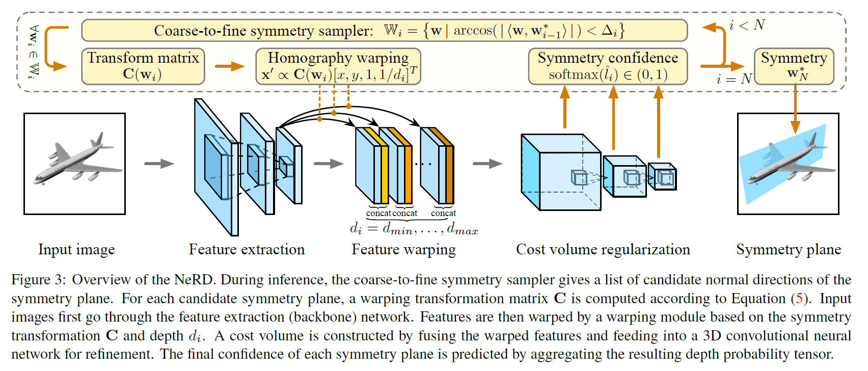
For the input image, first compute the 2D feature map, then generate a set of candidate symmetry plane normals. For each candidate normal \(\mathrm{w}\), warp the 2D feature map, construct a 3D cost volume for photo-consistency matching, and finally, the cost volume network converts the cost volume into confidence values, taking the \(\mathrm{w}\) with the highest confidence as the final predicted symmetry plane.

How to generate candidate symmetry plane normals? Since the domain of \(\mathrm{w}\), \(\mathbb{R}^3\), is continuous, brute-force sampling would be computationally expensive. Therefore, a coarse-to-fine strategy is adopted: first, sample uniformly, then find the \(\mathrm{w}^\star\) with the highest confidence, narrow the sampling range around \(\mathrm{w}^\star\), and iterate until the desired accuracy is achieved.

The feature extractor is a variant of ResNet. For each sampled \(\mathrm{w}\_i\), obtain its transformation matrix \(\mathrm{C}(\mathrm{w}\_i)\). For each pixel \((x, y)\) in the image, obtain its symmetric point \((x^{'}, y^{'})\), concatenate the features of these two pixels as feature warping, obtain the cost volume, and then feed the cost volume into the cost volume network (i.e., a series of 3D convolutions + max-pool + sigmoid) to get the confidence \(\hat{l}\_i\) for \(\mathrm{w}\_i\).

Training

At each level of the coarse-to-fine process, sample around the ground truth \(\mathrm{w}\). For each sampled \(\hat{\mathrm{w}}\), its label is:

The loss function is:

Applications

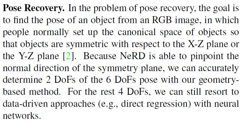
Pose Recovery

Not quite sure about the 2 DoFs here.

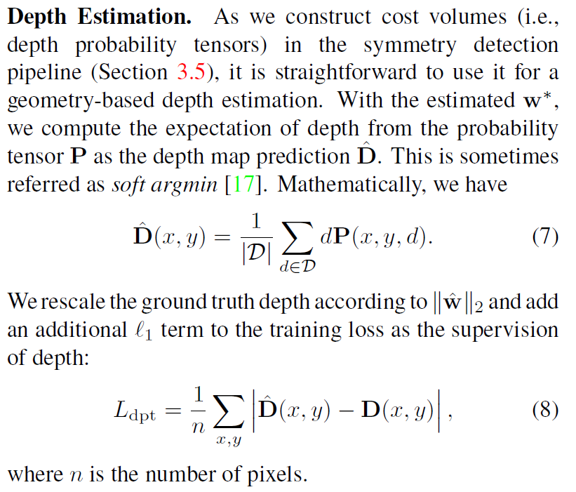
Depth Estimation